Learn how to draw and interpret a production possibility curve, calculate opportunity cost, and distinguish movements along the curve from shifts.
A production possibility curve (PPC) shows the maximum combinations of two goods an economy can produce in a given period with its available resources and technology. It is also called a production possibility frontier (PPF). Resources are limited, so producing more of one good can mean producing less of the other.
Read the axes and assumptions
Put the quantity of one good on each axis, with units and a time period. Here, the horizontal axis measures bicycles per day and the vertical axis measures loaves of bread per day.
For this simplified model:
- The economy produces only these two goods.
- The quantity and quality of resources and the available technology are fixed for the curve shown.
- Points on the frontier represent full and productively efficient use of resources.
- Resources can be moved between uses, but are not equally suited to both goods.
That last assumption explains why a PPC can bow outwards from the origin. As bicycle production expands, resources increasingly valuable for bread production must be transferred, so each additional bicycle costs more bread. A straight frontier would instead show constant opportunity cost.
A production possibilities schedule
Suppose an economy can produce these combinations:
| Point | Bicycles per day | Loaves of bread per day |
|---|---|---|
| A | 0 | 100 |
| B | 2 | 90 |
| C | 4 | 70 |
| D | 6 | 40 |
| E | 8 | 0 |
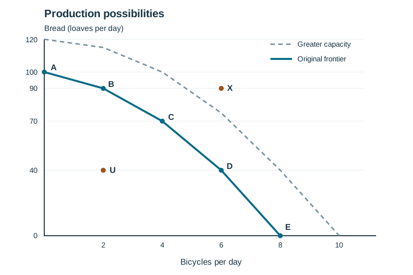
To draw this frontier, plot A to E using the table and join neighbouring points with straight line segments. The segments become steeper as bicycle output rises. They approximate a bowed-out curve; the table does not specify the exact shape between points.
Mark U at (2, 40), inside the frontier, and X at (6, 90), outside it. An additional frontier farther from the origin would represent greater productive capacity, rather than another combination available under the original conditions.
Calculate opportunity cost with units
Opportunity cost is the value of the next best alternative forgone. Here, measure the bread sacrificed to obtain more bicycles.
Moving from B to C increases bicycle output from 2 to 4 per day, while bread falls from 90 to 70 loaves per day.
Opportunity cost of the additional 2 bicycles = 20 loaves of bread.
Average opportunity cost per additional bicycle = 20 ÷ 2 = 10 loaves of bread per bicycle.
From C to D, the next 2 bicycles cost 30 loaves: an average of 15 loaves per bicycle. The cost rises as more resources move into bicycle production, giving the frontier its bowed-out shape. Keep the total cost of a movement separate from the average per bicycle. An interval average also need not equal the cost of each individual bicycle.
Distinguish a movement from a shift
B to C: movement along the frontier
Resources are reallocated towards bicycles. Productive capacity is unchanged, and bread output falls.
U to B: better use of existing capacity
At U, resources may be unemployed or used inefficiently. Moving to B increases bread output without sacrificing bicycles. The frontier does not shift. A point on it is productively efficient, but the diagram alone cannot tell us which combination society prefers.
An outward shift: greater productive capacity
More resources or improved technology can expand the combinations available. On a diagram, draw a new frontier outside the original one to show this change. A technological improvement benefiting only one industry may expand the frontier unevenly. X is unattainable under the original resources and technology; greater capacity can make it attainable later.
Explain a movement along the curve
"Making more bicycles shifts the curve because production increases" confuses higher output of one good with greater capacity. Describe what changes: "Moving from B to C increases bicycle output by 2 per day and reduces bread output by 20 loaves per day. This is a reallocation of existing resources along the frontier, with an average opportunity cost of 10 loaves per additional bicycle."
Check the opportunity cost
What is the average opportunity cost per additional bicycle when production moves from D to E?
Answer: Bread falls by 40 loaves and bicycle output rises by 2, so the cost is 40 ÷ 2 = 20 loaves per bicycle.
This guide is for Year 11 preparation, including students starting the new Economics syllabus in 2027. Their first HSC is in 2028; students sitting the HSC in 2027 continue on the 2009 syllabus. NESA's implementation timetable confirms the change. Our Economics syllabus guide explains the cohorts.
For help turning diagrams and calculations into clear explanations, explore Plume's Economics classes.